In recommendations setting, one would occasionally come across multi-armed bandits algorithm mentioned as a method to serve recommended content. In this article, I will go over what bandit algorithms mean, what the popular algorithms are, as well as how multi-armed bandits are used in recommendations.

Introduction to bandits algorithm

What is bandit?

Bandit refers to the slot machine in casino, where a gambler has to choose which machine (lever) to use that will maximize his probability of winning a reward.

Multi-armed bandit refers to the multiple machines a gambler will need to make decision on which sequence of the slot machines to use.

What is multi-armed bandit in ML?

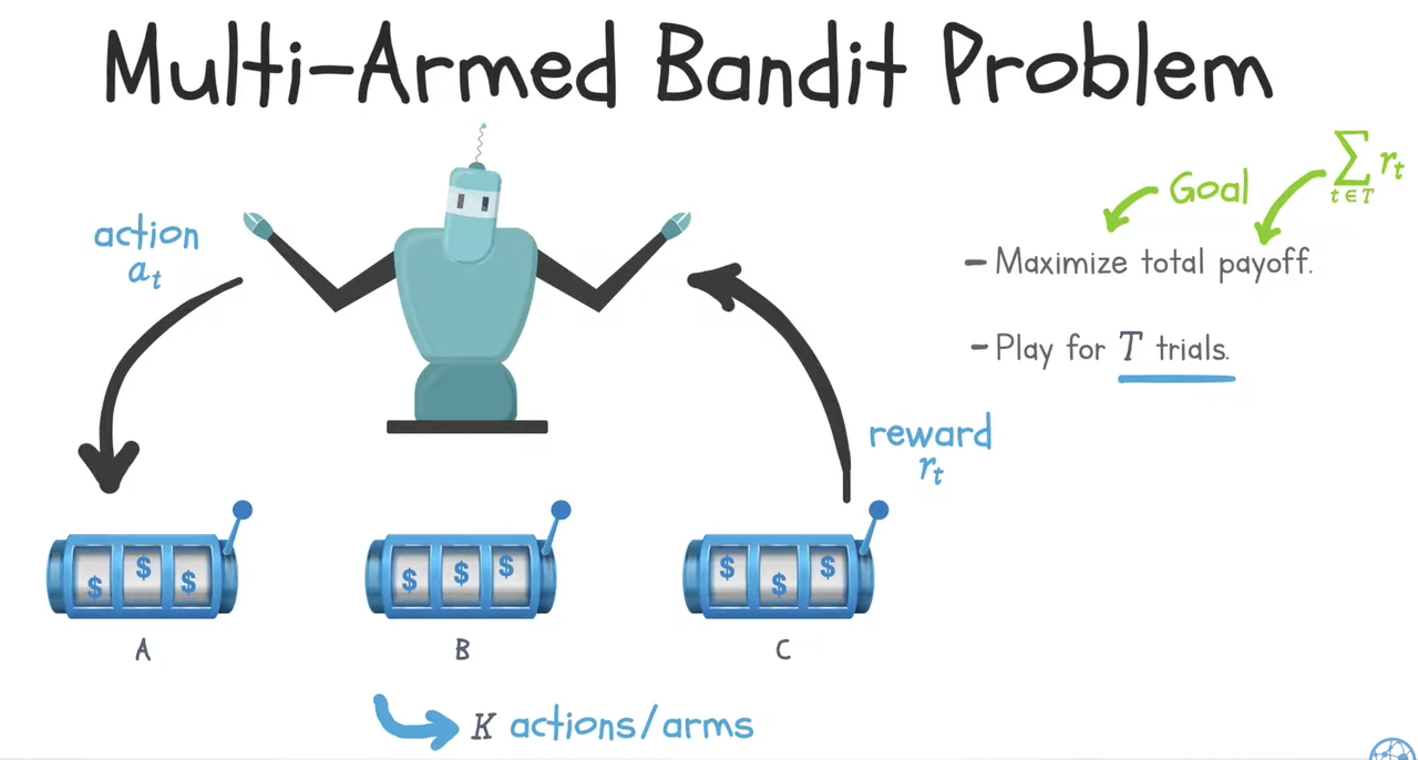
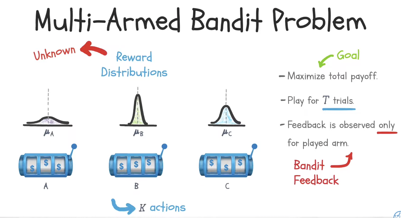
Multi-armed bandit problem (sometimes called the K- or N-armed bandit problem) is a problem in which a fixed limited set of resources must be allocated between choices in a way that maximizes their expected gain. Each choice’s properties are only partially known at the time of allocation, and may become better understood as time passes by. Multi-armed bandit is an algorithm within Reinforcement Learning, modelling exploration-exploitation trade off.

Multi-armed bandit algorithm in RecSys

In recommendation systems, we can use multi-armed bandit algorithm to sequentially select the candidates (ranking candidates) to maximize an objective (e.g. clicks, engagements, duration, revenue).

Recommenders tend to greedily promote items that received higher engagement in the past. This leads to popularity bias. With the explore-exploit nature of bandit algorithms, we can minimize such popularity bias by acknowledging the uncertainty in the data and deliberately exploring to reduce it.

In this talk, I will go through the common algorithms of multi-armed bandits and how it can be applied to recsys

Terminologies

(i) action/arm: recommendation candidates,

(ii) reward: customer interaction from a single trial, such as a click or purchase,

(iii) value: estimated long-term reward of an arm over multiple trials, and

(iv) policy: algorithm/agent that chooses actions based on learned values.

Types of bandits

1. ε-greedy

Epsilon-greedy is a classic bandit algorithm.

Algorithm:

The best candidate is selected for a proportion $1-\epsilon$ of the trials, and other candidates are selected at random (with uniform probability) for a proportion $\epsilon$.

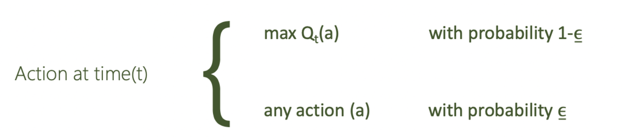
We pick the action with the top Q value with probability $1-\epsilon$ (exploit), and pick other action at random with probability $\epsilon$ (explore).

We balance the explore-exploit trade-off via the parameter ε. A higher ε leads to more exploration while a lower ε leads to more exploitation. A typical $\epsilon=0.1$

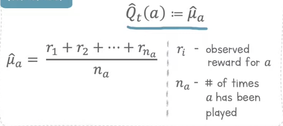
How to calculate $Q_t(a)$?

Q is the value function at time t for action a. Therefore, we can calculate Q as the average reward so far for taking action a

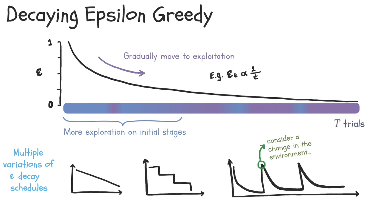
Decaying epsilon over time

As $\epsilon$ is the rate of exploration, if we are more confident of our best action, we can decay as there are more trials have been done

Advantages and disadvantages of epsilon-greedy

Advantages

• Simple to implement

Disadvantages

• Treat all exploration candidates the same (as we uniformly sample the actions in exploration stage). Some candidates are actually very bad, and do not need to be considered.

2. UCB (Upper Confidence Bound)

UCB considers the uncertainty of an arm and selects arms that have the highest potential. Uncertainty is modeled via confidence bounds while potential is represented by the upper confidence bound (thus the name of the algorithm)

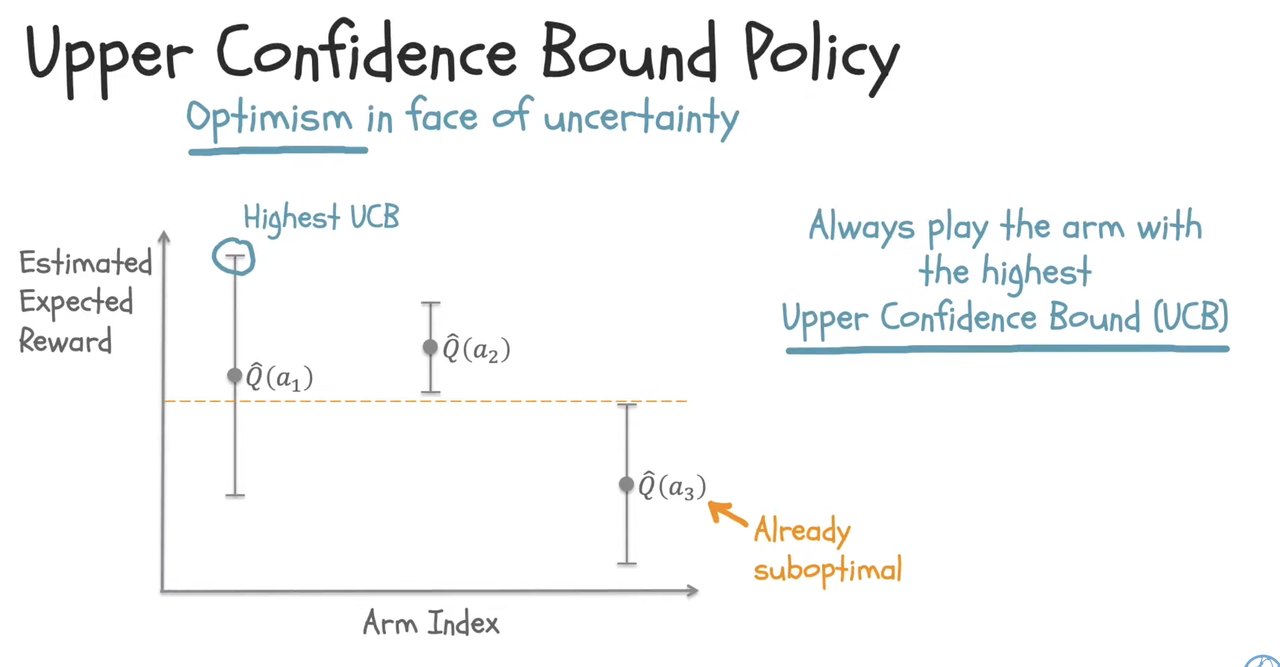
At each play, choose the action that has the highest upper confidence bound. Once we have its reward, we can update its confidence bound.

At time step t, every action will have the value $Q_t(a)$ and its “variance”. Upper confidence bound formula is:

$UCB(a_t) = Q_t(a) + ”variance”$

How to calculate $Q_t(a)$ and its “variance”?

$Q_t(a)$ is similar to epsilon-greedy $Q_t(a)$ which is the average reward for action a so far.

“variance” = $c\sqrt{\frac{log(t)}{N_{t-1}(a)}}$

Therefore,

$UCB(a_t) = Q_t(a) + variance$

$= \frac{\sum r_a}{N_{t-1}(a)} + c\sqrt{\frac{log(t)}{N_{t-1}(a)}}$

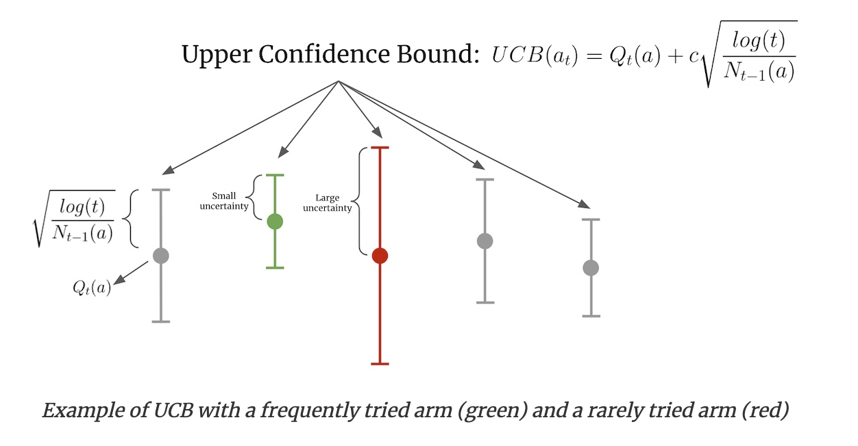
In the image above, Qₜ(a) is the estimated value of arm a at time step t, Nₜ(a) is the number of times arm a was selected, and c is a confidence parameter (which defaults to 1). The green arm has been chosen frequently and thus has narrower confidence bounds. In contrast, the red arm hasn’t been selected as often and thus has wider confidence bounds. When selecting an action, even though the green arm has a higher estimated value, the red arm has a higher UCB and is thus chosen. As the red arm is selected more, its confidence bounds will shrink. If the estimated value stays the same, its UCB will decrease to below the UCB of the green arm and the green arm will be chosen.

How to get $Q_t(a)$ at cold-start?

• Use UCB1: run through each action exactly once at the start to get Q value

Disadvantage of UCB approach

• Calculate $Q_t(a)$ through a frequentist approach (frequentist = average historical rewards). Can we model $Q_t(a)$ by using a probability distribution? That brings us to the next algorithm.

3. Thomson Sampling

Thomson Sampling models Q value by building a probability distribution from historical rewards and then samples from the distribution when choosing actions.

Assumed for each action that the reward is binary, a Bernoulli distribution is used:

$R_a \sim Bernoulli(p_a)$ where $R_a \in {0,1}$

When $R_a \sim Bernoulli$, due to conjugate property, if $Q_a=E(R_a)$, $Q_a$ follows Beta distribution

$Q_a \sim Beta(\alpha, \beta)$

The Beta distribution takes two parameters, α and β, and the mean value of the distribution is α/(α + β) which can be thought of as successes / (successes + failures)

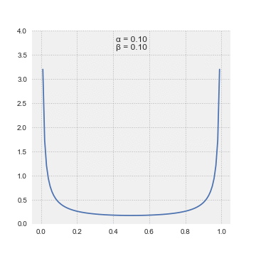
To select an action, we sample from each arm’s Beta distribution and choose the arm with the highest sampled values.

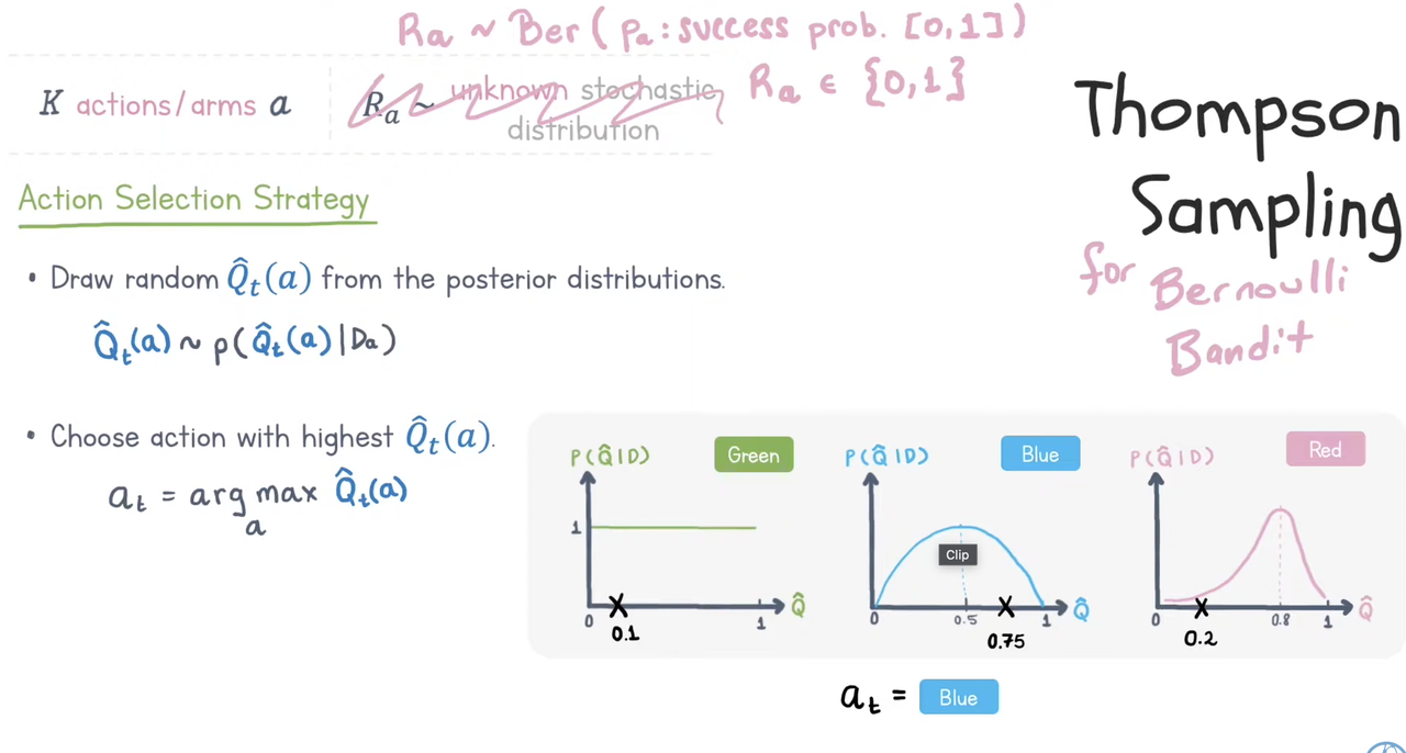
How to update $Q_t(a)$ after you have the reward signal?

Update the Beta distribution according to successes and failures.

$Q_a \sim Beta(\alpha, \beta)$ where $\alpha$ is number of successes, and $\beta$ is number of failures

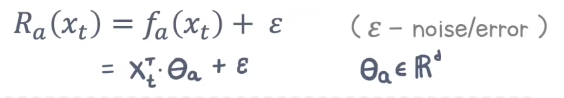
4. LinUCB

LinUCB is a type of contextual bandit that uses linear regression to approximate reward.

What is contextual bandit?

Contextual bandit refers to the type of bandit algorithm that makes use of a contextual input vector. For example, in the case of recsys, a user profile or content profile is a context.

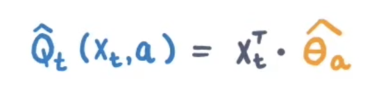
LinUCB algorithm

LinUCB learns a least-square ridge regression to predict reward based on context vector:

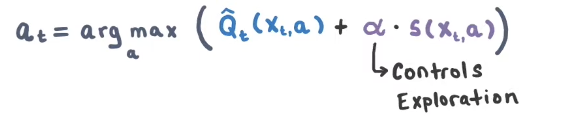
Q value is approximated using the learned parameters:

Action is picked based on the highest Q value, plus a control exploration term

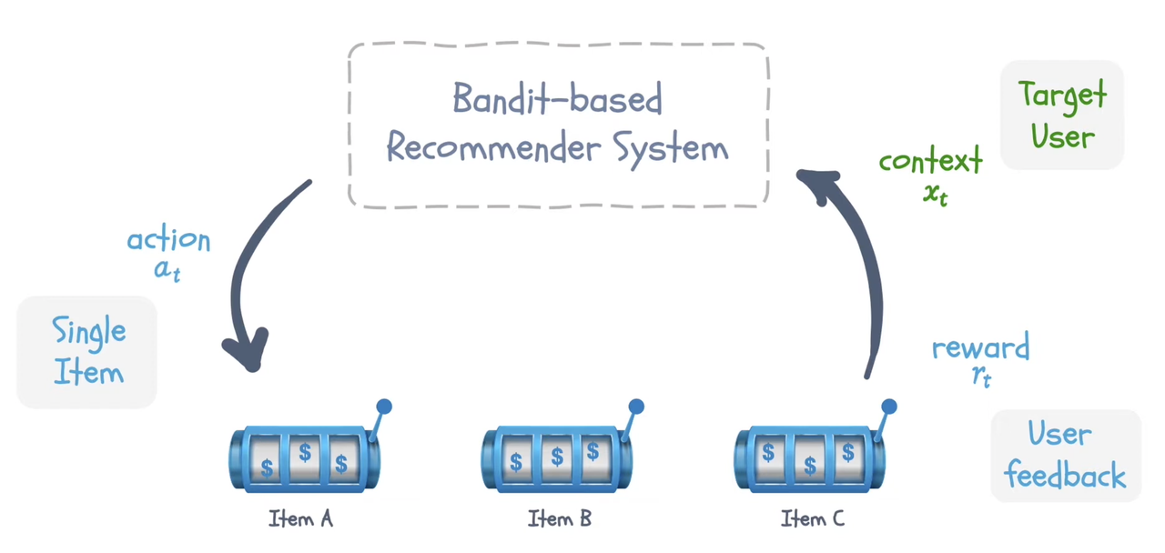
Bandits setup in Recommendation Systems

In recommendation settings, each item to recommend is a bandit arm or action. Reward is clicks, or engagements. Context is the user vector.

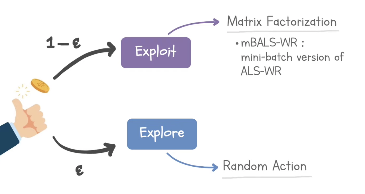
1. ε-greedy

• Exploit $1-\epsilon$: matrix factorization

• Explore $\epsilon$: random action

Papers: Large-Scale Parallel Collaborative Filtering for the Netflix Prize

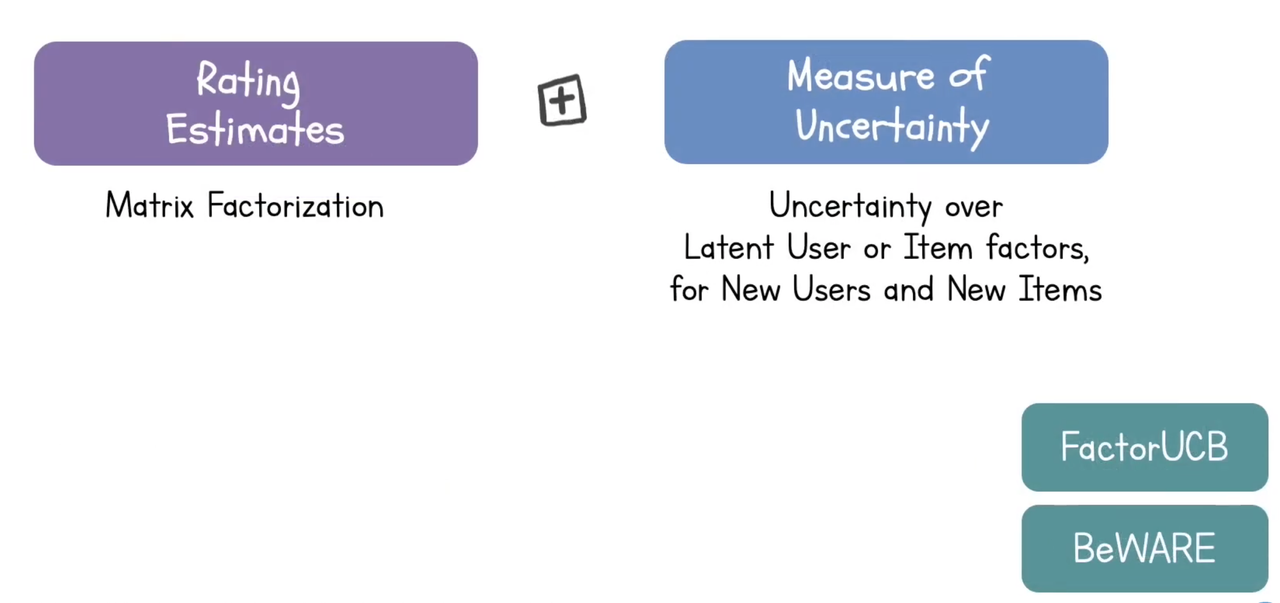
2. UCB

• Exploit: rating estimates using matrix factorization

• Exploration: uncertainty over latent user or item factors

Papers: FactorUCB, BeWARE

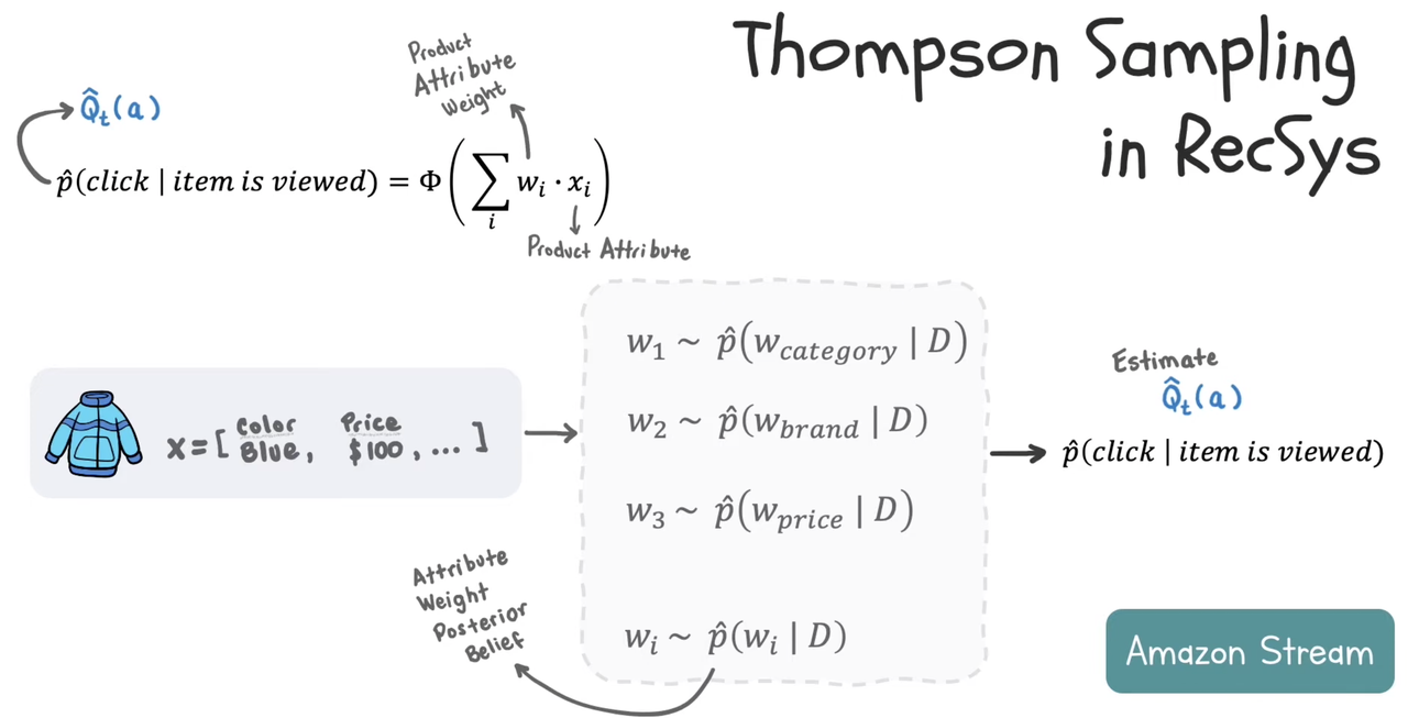
3. Thomson Sampling

• Model p(click | item) based on weighted sum of each product attribute

• Weight is sampled from posterior distribution after observing the data

4. Recommending lists

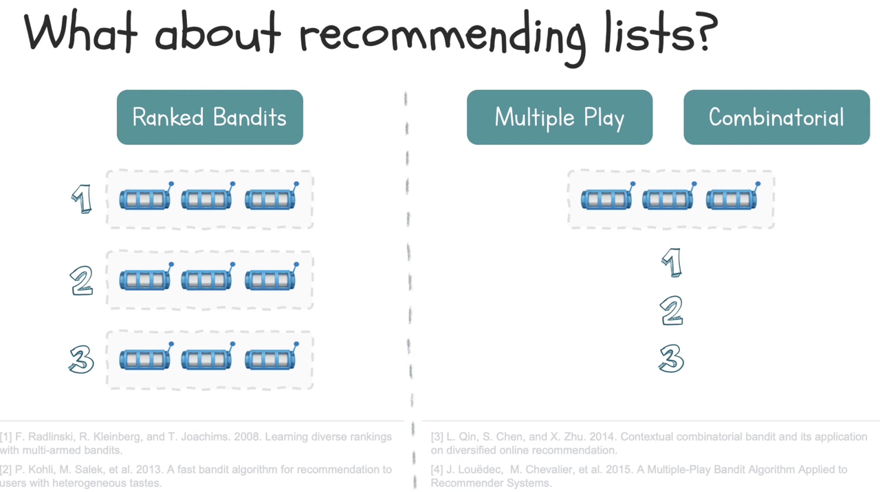
• Ranked bandits: each position in the list has a separate bandit

• Multiple play: choose multiple actions at one time

• Combinatorial: each bandit consists of a list of items

Reference

Bandits for Recommender Systems

RecSys 2020 Tutorial: Introduction to Bandits in Recommender Systems